A Consensus-Based Algorithm for Non-Convex Multiplayer Games: Nonlinear Oligopoly Games

Table of Links

Abstract and 1 Introduction

2 Global convergence

2.1 Quantitative Laplace principle

2.2 Global convergence in mean-field law

3 Numerical experiments and 3.1 One-dimensional illustrative example

3.2 Nonlinear oligopoly games with several goods

4 Conclusion, Acknowledgments, Appendix, and References

3.2 Nonlinear oligopoly games with several goods

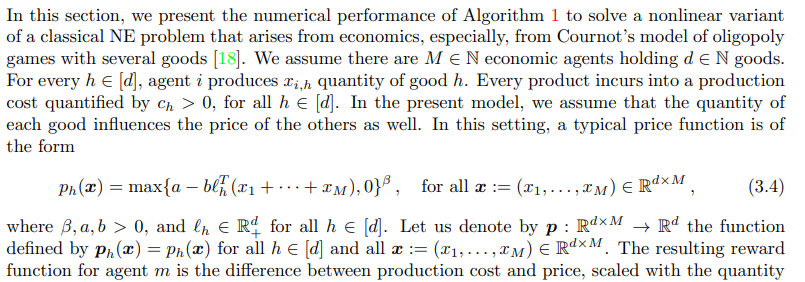
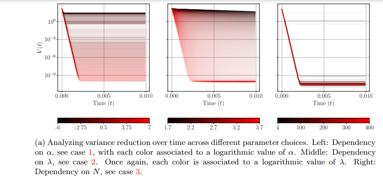
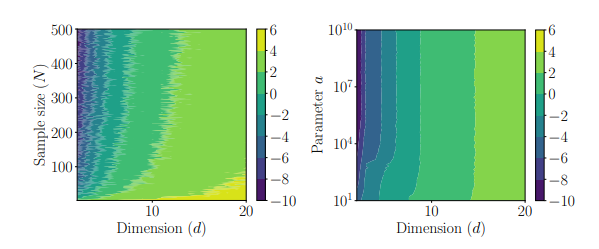
Figure 2: Studying the dependence of Algorithm 1 with respect to the algorithm’s parameters to solve (3.5).

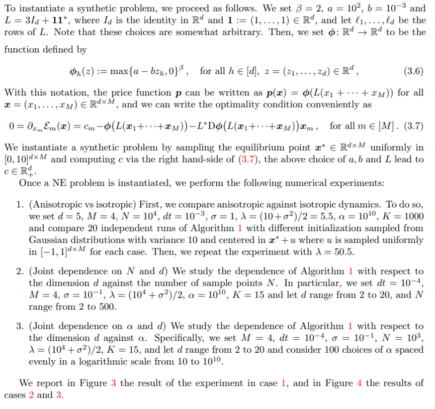
of good produced, namely

3.2.1 Experimental setup

3.2.2 Results and discussio

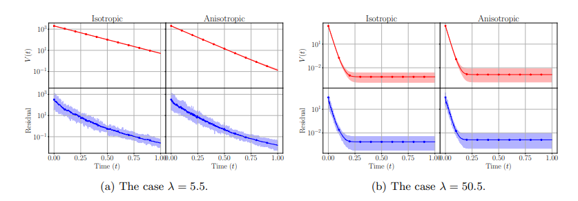
In Figure 3, which shows the results corresponding to the experiment in case 1, as observed for instance in [28], we see that the anisotropic case does indeed show a faster convergence rate especially in the initial iterations and for λ which is of the order of σ 2 . If λ increases, though, we see no significant differences in the convergence behavior of anisotropic or isotropic dynamics, both for the residual and for the variance decrease.

Figure 4 shows the results of the comparisons in cases 3 and 2. Regarding case 2, we can see that indeed as the dimension increases, we need exponentially many particles (quantified by N) to reach high accuracy of order 10−9 . This indicates that Algorithm 1, while being quite reliable, and sometimes the only available solver for low-dimensional problems, might need further improvement in high-dimensional settings.